Part 3 – Configuring Hardware and Hard Disks
July 11, 2017Configuring Hardware
Exam Objectives
- 101.1 – Determine and configure hardware settings
- 102.1 – Design hard disk layout
- 104.1 – Create partitions and filesystems
- 104.2 – Maintain the integrity of filesystems
- 104.3 – Control mounting and unmounting of filesystems
Configuring the Firmware and Core Hardware
Firmware is the lowest level software that runs on a computer. A computer’s firmware begins the boot process and configures certain hardware devices.
Key components managed by the firmware (and Linux, once it’s booted) include interrupts, I/O addresses, DMA addresses, the real-time clock, and Advanced Technology Attachment (ATA) hard disk interfaces.
Understanding the Role of the Firmware
Many types of firmware are installed on the various hardware devices found inside a computer, but the most important firmware is on the motherboard.
In the past, most x86 and x86_64 based computers had a firmware known as the Basic Input/Output System (BIOS). Since 2011, however, Extensible Firmware Interface (EFI) and it’s successor, Unified EFI (UEFI), has become the standard.
Note: While most x86 and x86_64 computers use a BIOS or EFI, some computers may use other software in place of these types of firmware. For example, old PowerPC-based Apple computers use OpenFirmware.
Despite the fact that EFI isn’t a BIOS, most manufacturers refer to it by that name in their documentation. Additionally, the the exam objectives refer to the BIOS, but not EFI.
The motherboard’s firmware resides in electronically erasable programmable read-only memory (EEPROM), aka flash memory.
When a computer is turned on, the firmware performs a power-on self-test (POST), initializes hardware to a known operational state, and loads the boot loader from the boot device (typically the first hard disk), and passes control onto the boot loader — which in turn loads the operating system.
Most BIOSs and EFIs provide an interactive interface to configure them — typically found by pressing the Delete key or a Function key during the boot sequence.
Note: Many computers prevent booting if a keyboard is unplugged. To disable this, look for a firmware option called Halt On or similar with the BIOS or EFI.
Once Linux boots, it uses its own drivers to access the computer’s hardware.
Note: Although the Linux kernel uses the BIOS to collect information about the hardware of a machine, once Linux is running, it doesn’t use BIOS services for I/O. As of the 3.5.0 kernel, Linux takes advantages of a few EFI features.
IRQs
An interrupt request (IRQ), or interrupt, is a signal sent to the CPU instructing it to suspend its current activity and handle some external event, such as keyboard input.
On the x86 platform, 16 IRQs are available — numbered 0 to 15. Newer systems, including x86_64 systems, have an even greater number of IRQs.
IRQs and their common uses:
| Command | Typical Use | Notes |
0 |
System Timer | Reserved for internal use. |
1 |
Keyboard | Reserved for keyboard use only. |
2 |
Cascade for IRQs 8 — 15 |
The original x86 IRQ-handling circuit can manage just 8 IRQs; two sets of these are tied together to handle 16 IRQs, but IRQ 2 must be used to handle IRQs 8 — 15 |
3 |
Second RS-232 serial port ( COM2: in Windows) |
May also be shared by a fourth RS-232 serial port. |
4 |
First RS-232 serial port ( COM1: in Windows) |
May also be shared by a third RS-232 serial port. |
5 |
Sound card or second parallel port ( LPT2: in Windows) |
|
6 |
Floppy disk controller | Reserved for the first floppy disk controller. |
7 |
First parallel port ( LPT1: in Windows) |
|
8 |
Real-time clock | Reserved for system clock use only. |
9 |
ACPI system control interrupt | Used by Intel chipsets for the Advanced Configuration and Power Interface (ACPI) used for power management. |
10 |
Open interrupt | |
11 |
Open interrupt | |
12 |
PS/2 mouse | |
13 |
Math coprocessor | Reserved for internal use. |
14 |
Primary ATA controller | The controller for ATA devices such as hard drives; traditionally /dev/hda and /dev/hdb under Linux. |
15 |
Secondary ATA controller | The controller for additional ATA devices; traditionally /dev/hdc and /dev/hdd under Linux. |
Note: Most modern distributions treat Serial ATA disks as SCSI disks, which changes their device identifiers from /dev/hdx to /dev/sdx.
The original Industry Standard Architecture (ISA) bus design (which has become rare on computers since 2001) makes sharing an interrupt between two devices tricky. Therefore, it is ideal that every ISA device should have it’s own IRQ.
The more recent Peripheral Component Interconnect (PCI) bus makes sharing interrupts a bit easier, so PCI devices frequently end up sharing an IRQ.
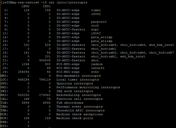
Once a Linux system is running, you can explore what IRQs are being used for various purposes by examining the contents of the /proc/interrupts file:
$ cat /proc/interrupts
Example from CentOS 6.9:
Note: The /proc filesystem is a virtual filesystem — it refers to kernel data that’s convenient to represent using a filesystem, rather than actual files on a hard disk.
The above example output shows the IRQ number in the first column. The next two columns show each CPU core and the number of interrupts each has received for that particular IRQ. The column after them reports the type of interrupt, followed by the name of the device that is located at that IRQ.
Note: The /proc/interrupts file lists IRQs that are in use by Linux, but Linux doesn’t begin using an IRQ until the relevant driver is loaded. This may not happen until you attempt to use the hardware. As such, the /proc/interrupts list may not show all of the interrupts that are configured on your system.
Although IRQ conflicts are rare on modern hardware, they still do occasionally happen. When this occurs, you must reconfigure one or more devices to use different IRQs.
I/O Addresses
I/O addresses (aka I/O ports) are unique locations in memory that are reserved for communications between the CPU and specific physical hardware devices.
Like IRQs, I/O addresses are commonly associated with specific devices, and they should not ordinarily be shared.
Common Linux devices, along with their typical IRQ number and I/O addresses:
| Linux Device | Typical IRQ | I/O Address | Windows Name |
/dev/ttyS0 |
4 |
0x03f8 |
COM1 |
/dev/ttyS1 |
3 |
0x02f8 |
COM2 |
/dev/ttyS2 |
4 |
0x03e8 |
COM3 |
/dev/ttyS3 |
3 |
0x02e8 |
COM4 |
/dev/lp0 |
7 |
0x0378 - 0x037f |
LPT1 |
/dev/lp1 |
5 |
0x0278 - 0x027f |
LPT2 |
/dev/fd0 |
6 |
0x03f0 - 0x03f7 |
A: |
/dev/fd1 |
6 |
0x0370 - 0x0377 |
B: |
Note: Although the use is deprecated, older systems sometimes use /dev/cuax (where x is a number 0 or greater) to indicate an RS-232 serial device. Thus, /dev/ttyS0 and /dev/cua0 refer to the same physical device.
Once a Linux system is running, you can explore what I/O addresses the computer is using by examining the contents of the /proc/ioports file:
$ cat /proc/ioports
jeff@mg-rex-mint ~ $ cat /proc/ioports
0000-0cf7 : PCI Bus 0000:00
0000-001f : dma1
0020-0021 : pic1
0040-0043 : timer0
0050-0053 : timer1
0060-0060 : keyboard
0061-0061 : PNP0800:00
0064-0064 : keyboard
0070-0071 : rtc0
0080-008f : dma page reg
[...truncated...]
DMA Addresses
Direct memory addressing (DMA) is an alternative method of communication to I/O ports. Rather than have the CPU mediate the transfer of data between a device and memory, DMA permits the device to transfer data directly, without the CPU’s attention.
To learn what DMA channels your system uses:
$ cat /proc/dma
jeff@mg-rex-mint ~ $ cat /proc/dma
4: cascade
The above output indicates that DMA channel 4 is in use. As with IRQs and I/O ports, DMA addresses should not be shared normally.
Boot Disks and Geometry Settings
BIOS
The BIOS boot process begins with the computer reading a boot sector (typically the first sector) from a disk and then executing the code contained within it.
This limits boot options for BIOS-based computers to only selecting the order in which various boot devices (hard disks, optical disks, USB devices, network boot, etc.) are examined for a boot sector.
EFI
Under EFI, the boot process involves the computer reading a boot loader file from a filesystem on a special partition, known as the EFI System Partition (ESP). This file can take a special default name or it can be registered in the computer’s NVRAM.
This allows EFI computers to have an extended range of boot options, involving both default boot loader files from various devices and multiple boot loaders on the computer’s hard disks.
Note: Many EFI implementations support a BIOS compatibility mode, and so they can boot media intended for BIOS-based computers.
Booting Options
Some viruses are transmitted by BIOS boot sectors. As such, it’s a good idea not to make booting from removable media the first priority; it’s better to make the first hard disk (or boot loader on a hard disk’s ESP, in the case of EFI) the only boot device.
Note: The Windows A: floppy disk is /dev/fd0 under Linux.
In most cases, the firmware detects and configures hard disks and CD/DVD drives correctly. In rare circumstances, you must tell a BIOS-based computer about the hard disk’s cylinder / head / sector (CHS) geometry.
Cylinder / Head / Sector (CHS) Geometry
The CHS geometry is a holdover from the early days of the x86 architecture. A traditional hard disk layout consist of a fixed number of read/write heads that can move across the disk surfaces / platters. As the disk spins, each head marks out a circular track on its platter. These tracks collectively make up a cylinder. Each track is broken down into a series of sectors.
Any sector on a hard disk can be uniquely identified by three numbers: a cylinder number, a head number, and a sector number.
The x86 BIOS was designed to use the three number CHS identification code — requiring the BIOS to know how many cylinders, heads, and sectors the disk has. Most modern hard disks relay this information to the BIOS automatically, but for compatibility with the earliest hard disks, BIOSs still enable you to set these values manually.
Note: The BIOS will detect only certain types of disks. Of particular importance, SCIS disks and SATA disks won’t appear in the main BIOS disk-detection screen. These disks are handled by supplementary firmware associated with the controllers for these devices. Some BIOSs do provide explicit options to add SCSI devices into the boot sequence, which allows you to give priority to either ATA or SCSI devices. For BIOSs without these options, SCSI disks are generally given less priority than ATA disks.
The CHS geometry presented to the BIOS of a hard disks is a convenient lie — as most modern disks squeeze more sectors onto the outer tracks than the inner ones for greater storage capacity.
Plain CHS geometry also tops out at 504 MiB, due to the limits on the numbers in the BIOS and in the ATA hard disk interface.
Note: Hard drive sizes use the more accurate mebibyte (MiB) size instead of the standard megabyte (MB). In general use, most people will say megabyte when actually referencing the size of a mebibyte (likewise for gigabyte and gibibyte). It’s 1000 MB to 1 GB, whereas it’s 1024 MiB to 1 GiB.
Various patches, such as CHS geometry translation, can be used to expand the limit to about 8 GiB. However, the preference these days is to use logical/linear block addressing (LBA) mode.
In LBA mode, a single unique number is assigned to each sector on the disk, and the disk’s firmware is smart enough to read from the correct head and cylinder when given this sector number.
Modern BIOSs typically provide an option to use LBA mode, CHS translation mode, or possibly some other modes with large disks. EFI uses LBA mode exclusively, and doesn’t use CHS addressing at all (except for BIOS compatibility mode).
Coldplug and Hotplug Devices
Hotplug devices can be attached and detached when the computer is turned on (i.e. “hot”). Coldplug devices must be attached and detached when the computer is in an off state (i.e. “cold”).
Note: Attempting to attach or detach a coldplug device when the computer is running can damage the device or the computer.
Traditionally, components that are internal to the computer, such as CPU, memory, PCI cards, and hard disks, have been coldplug devices. A hotplug variant of PCI does exist, but it’s mainly on servers and other systems that can’t afford downtime required to install or remove a device. Hotplug SATA devices are also available.
Modern external devices, such as Ethernet, USB, and IEEE-1394 devices, are hotplug. These devices rely on specialized Linux software to detect the changes to the system as they’re attached and detached. Several utilities help with managing hotplug devices:
Sysfs
The sysfs virtual filesystem, mounted at /sys, exports information about devices so that user-space utilities can access the information.
Note: A user space program is one that runs as an ordinary program, whether it runs as an ordinary user or as root. This contrasts with kernel space code, which runs as part of the kernel. Typically only the kernel (and hence kernel-space code) can communicate directly with hardware. User-space programs are ultimately the users of hardware, though. Traditionally the /dev filesystem has provided the main means of interface between user space programs and hardware.
HAL Daemon
The Hardware Abstraction Layer (HAL) Daemon, or hald, is a user-space program that runs at all times and provides other user-space programs with information about available hardware.
D-Bus
The Desktop Bus (D-Bus) daemon provides a further abstraction of hardware information access. D-Bus enables processes to communicate with each other as well as to register to be notified of events, both by other processes and by hardware (such as the availability of a new USB device).
udev
Traditionally, Linux has created device nodes as conventional files in the /dev directory tree. The existence of hotplug devices and various other issues, however, have motivated the creation of udev — a virtual filesystem, mounted at /dev, which creates dynamic device files as drivers are loaded and unloaded.
udev can be configured through files located at /etc/udev, but the standard configuration is usually sufficient for common hardware.
Older external devices, such as parallel and RS-232 ports, are officially coldplug in nature. When RS-232 or parallel port devices are hotplugged, they typically aren’t registered by tools such as udev and hald. The OS handles the ports to which these devices connect; so it’s up to user space programs, such as terminal programs and/or the printing system, to know how to communicate with the external devices.
Configuring Expansion Cards
Many hardware devices require configuration — the IRQ, I/O port, and DMA addresses used by the device must be set. In the past, such things were set using physical jumpers. Presently, most devices can be configured via software.
Configuring PCI Cards
The PCI bus, which is the standard expansion bus for most internal devices, was designed with Plug-and-Play (PnP) style configuration in mind, thus automatic configuration of PCI devices is the rule rather than the exception.
In general, PCI devices configure themselves automatically, and there is no need to make any changes. However, it is possible to tweak how PCI devices are detected in several ways:
- The Linux kernel has several options that affect how it detects PCI devices. These can be found in the kernel configuration screens under Bus Options. Most users can rely on the options in their distributions’ default kernel to work properly; but if the kernel was recompiled by yourself, and you are experiencing problems with device detection, these options may need to be adjusted.
- Most firmware implementations have PCI options that change the way PCI resources are allocated. Adjusting these options may help if strange hardware problems occur with PCI devices.
- Some Linux drivers support options that cause them to configure the relevant hardware to use particular resources. Details of these options can often be found in the drivers’ documentation files. These options must be passed to the kernel using a boot loader or kernel module options.
- The
setpciutility can be used to query and adjust PCI devices’ configurations directly. This tool can be useful if you know enough about the hardware to fine-tune its low-level configuration; but it’s not often used to tweak the hardware’s basic IRQ, I/O port, or DMA options.
To check how PCI devices are currently configured, the lspci command can be used to display all of the information about the PCI busses on your system and all of the devices connect to those busses.
Common lspci options:
| Option | Description |
-v |
Increases verbosity of output. This option can be doubled ( -vv) or tripled (-vvv) to produce even more output. |
-n |
Displays information in numeric codes rather than translating the codes to manufacturer and device names. |
-nn |
Displays both the manufacturer and devices names along with their associated numer codes. |
-x |
Displays the PCI configuration space for each device as a hexadecimal dump. This is an extremely advanced option. Tripling ( -xxx) or quadrupling (-xxxx) this option displays information about more devices. |
-b |
Shows IRQ numbers and other data as seen by devices rather than as seen by the kernel. |
-t |
Displays a tree view, depicting the relationship between devices. |
-s [[[[domain]:]bus]:][slot][.[func]] |
Displays only devices that match the listed specification. This can be used to trim the results of the output. |
-d [vendor]:[device] |
Shows data on the specified device. |
-i <file> |
Uses the specified file to map vendor and device IDs to names. (The default is /usr/share/misc/pci.ids). |
-m |
Dumps data in a machine-readable form intended for use by scripts. A single -m uses a backward-compatible format, whereas doubling (-mm) uses a newer format. |
-D |
Displays PCI domain numbers. These numbers normally aren’t displayed. |
-M |
Performs a scan in bus-mapping mode, which can reveal devices hidden behind a misconfigured PCI bridge. This is an advanced option that can be used only by root. |
--version |
Displays version information. |
Learning about Kernel Modules
Kernel drivers, many of which come in the form of kernel modules, handle hardware in Linux.
Kernel modules are stand-alone driver files, typically stored in the /lib/modules directory tree, that can be loaded to provide access to hardware and unloaded to disable such access. Typically, Linux loads the modules it needs when it boots, but you may need to load additional modules yourself.
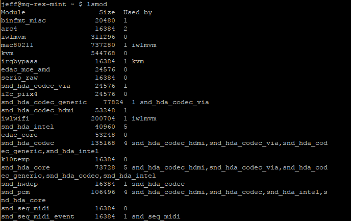
The lsmod command can be used to display the modules that are currently loaded:
$ lsmod
Example output:
[...truncated...]
The above output has several columns:
- The first column is labeled
moduleand represents the name of module currently loaded. To learn more about these modules, use themodinfocommand. - The
Sizecolumn shows how much memory is consumed by the module. - The
Used Bycolumn has a number to represent how many other modules or processes are using that module, followed by a list of those modules/processes. If the number is0it is not currently in use.
Note: The lsmod command displays information only about kernel modules, not about drivers that are compiled directly into the Linux kernel. For this reason, a module may need to be loaded on one system but not on another to use the same hardware, because the second system may compile the relevant driver directly into the kernel.
To find out more details about a particular module, use the modinfo command:
$ modinfo <module-name>
Loading Kernel Modules
Linux enables you to load kernel modules with two programs:
insmodmodprobe
The insmod program inserts a single module into the kernel. This process requires that all dependencies for this module be loaded beforehand.
The modprobe program accomplishes the same actions, but loads the dependencies automatically.
Note: In practice, you may not need to use insmod or modprobe to load modules because Linux can load them automatically. This ability relies on the kernel’s module autoloader feature, which must be compiled into the kernel, and on various configuration files, which are also required for modprobe and some other tools. Using insmod and modprobe can be useful for testing new modules or for working around problems with the autoloader, though.
The insmod command accepts a module filename:
# insmod /lib/modules/3.0.19/kernel/drivers/bluetooth/bluetooth.ko
The modprobe command accepts a module name instead of a filename:
# modprobe bluetooth
Note: modprobe relies on a configuration file at /etc/modprobe.conf or multiple configuration files within /etc/modprobe.d/ to use module names instead of filenames.
There are several options/features for modprobe:
| Feature | Option | Description |
| Be Verbose |
|
Tells modprobe to display extra information about its operations.Typically, this includes a summary of every insmod operation it performs. |
| Change Configuration Files | -C <filename> |
Change the configuration file or directory. |
| Perform a Dry Run | -n--dry-run |
Causes modprobe to perform checks and all other operations except the actual module insertions.This option can be used in conjunction with -v to see what modprobe would do without actually loading the module. |
| Remove Modules | -r--remove |
Reverses modprobe‘s usual effect. It removes the module and any on which it depends (unless those dependencies are in use by other modules). |
| Force Loading | -f--force |
Force the module loading, even if the kernel version doesn’t match what the module expects. This can occassionally be required when using third-party binary-only modules. |
| Show Dependencies | --show-depends |
Shows all modules on which a specific module depends (i.e. module dependencies). Note: This option doesn’t install any of the modules, it only provides information. |
| Show Available Modules | -l--list |
Displays a list of available options whose names match the wildcard specified. For example: Note: If no wildcard is provided, all available modules are displayed. Additionally, this option does not actually install any modules. |
Consult man modprobe for additional options.
Viewing Loaded Module Options
A loaded module has its options/parameters available at:
/sys/module/<module-name>/parameters/<parameter-name>
Removing Kernel Modules
In most cases, modules can be loaded indefinitely; the only harm that a module does when it’s loaded but not used is consume a small amount of memory.
Reasons for removing a loaded module can include: reclaiming a tiny amount of memory, unloading an old module so that an updated replacement can be loaded, and removing a module that is suspected to be unreliable.
The rmmod command can be used to unload a kernel module by name:
# rmmod bluetooth
There are several options/features for rmmod:
| Feature | Option | Description |
| Be Verbose |
|
Causes rmmod to display extra information about its operations. |
| Force Removal | -f--force |
Forces module removal, even if the module is marked as being in use. This option has no effect unless the CONFIG_MODULE_FORCE_UNLOAD kernel option is enabled. |
| Wait Until Unused | -w--wait |
Causes rmmod to wait for the module to become unused. Once the module is no longer being used, rmmod unloads the module.Note: rmmod doesn’t return anything until it unloads a module, which can make it look like it’s not doing anything. |
Consult man rmmod for additional options.
Like insmod, rmmod operates on a single module. If an attempt is made to unload a module that’s in use or depended on by other modules, an error message will be displayed. If other modules depend on the module, rmmod lists those modules — making it easier to decide whether to unload them or not.
To unload an entire module stack (a module and all of its dependencies) use the modprobe command with it’s -r option.
Configuring USB Devices
USB Basics
USB is a protocol and hardware port for transferring data to and from devices. It allows for many more (and varied) devices per interface port than either ATA or SCSI, and it gives better speed than RS-232 serial and parallel ports.
- The USB 1.0 and 1.1 specification allow for up to 127 devices and 12Mbps of data transfer.
- USB 2.0 allows for up to 480Mbps of data transfer.
- USB 3.0 supports a theoretical maximum speed of 4.8Gbps, although 3.2Gbps is more likely its top speed in practice. In addition, it also uses a different physical connector than 1.0, 1.1, and 2.0 connectors. USB 3.0 connectors can accept 2.0, 1.1, and 1.0 devices however.
Note: Data transfer speeds may be expressed in bits per second (bps) or multiples thereof, such as megabits per second (Mbps) or gigabits per second (Gbps). Or they can be expressed in bytes per second (Bps) or multiples thereof, such as megabytes per second (MBps). In most cases, there are 8 bits per bytes, so multiplying or dividing by 8 may be necessary to compare devices using different measurements.
Most computers ship with several USB ports. Each port can handle one device itself, but a USB hub can also be used to connect several devices to each port.
Linux USB Drivers
Several different USB controllers are available, with names such as UHCI, OHCI, EHCI, and R8A66597.
Modern Linux distributions ship with the drivers for the common USB controllers enabled, so the USB ports should be activated automatically when the computer is booted.
The UHCI and OHCI controllers handle USB 1.x devices, but most other controllers can handle USB 2.0 devices. A kernel of 2.6.31 or greater is required to use USB 3.0 hardware.
Note: These basic USB controllers merely provide a means to access the actual USB hardware and address the devices in a low-level manner. Additional software (either drivers or specialized software packages) will be needed to make practical use of the devices.
The lsusb utility can be used to learn more about USB devices:
$ lsusb
Example output:
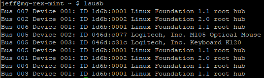
The above output shows seven USB busses are detected (001 – 007). Only the fifth bus (005) shows devices attached — a Logitech mouse and keyboard. These devices have a vendor ID of 046d and product IDs of c007 and c31c, respectively.
Note: The IDs for each device can be used to look up what device they are. This is especially helpful if they have a vague description.
There are several options for lsusb:
| Feature | Option | Description |
| Be Verbose |
|
Produces extended information about each device. |
| Restrict Bus and Device Number | -s [[bus]:][devnum] |
Restricts the output to the specified bus and device number. |
| Restrict Vendor and Product | -d [vendor]:[product] |
Limits the output to a particular vendor and product.vendor and product are the codes just after the ID on each line of the basic output. |
| Display Device by Filename | -D <filename> |
Displays information about the device that’s accessible via <filename>, which should be a file in the /proc/bus/usb directory tree.This directory provides a low-level interface to USB devices. |
| Tree View | -t |
Displays the device list as a tree. This makes it easier to see which devices are connected to which controllers. |
| Version | -V--version |
Displays the version of the lsusb utility. |
Note: Early Linux USB implementations required separate drivers for every USB device. Many of these drivers remain in the kernel, and some software relies on them. For instance, USB disk storage devices use USB storage drivers that interface with Linux’s SCSI support, making USB hard disks, removable disks, and so on look like SCSI devices.
Linux provides a USB filesystem that in turn provides access to USB devices in a generic manner. This filesystem appears as part of the /proc virtual filesystem.
In particular, USB device information is accessible from /proc/bus/usb. Subdirectories of /proc/bus/usb are given numbered names based on the USB controllers instead of the computer, as in /proc/bus/usb/001 for the first USB controller.
USB Manager Applications
USB can be challenging for OSs because it was designed as a hot-pluggable technology. The Linux kernel wasn’t originally designed with this sort of activity in mind, so the kernel relies on external utilities to help manage matters. Two tools in particular are used for managing USB devices: usbmgr and hotplug.
Note: While these tools are not commonly installed by default in Linux distributions, they can come in handy when working with USB devices.
The usbmgr package (located at http://freecode.com/projects/usbmgr) is a program that runs in the background to detect changes on the USB bus. When it detects changes, it loads or unloads the kernel modules that are required to handle the devices. This package uses configuration files in /etc/usbmgr to handle specific devices and uses /etc/usbmgr/usbmgr.conf to control the overall configuration.
With a shift from in-kernel device-specific USB drivers to the USB device filesystem (/proc/bus/usb), usbmgr has been declining in importance.
Instead of usbmgr, most distributions rely on the Hotplug package (http://linux-hotplug.sourceforge.net), which relies on kernel support added with the 2.4.x kernel series.
The Hotplug system uses files stored in /etc/hotplug to control the configuration of specific USB devices. In particular, /etc/hotplug/usb.usermap contains a database of USB device IDs and pointers to scripts in /etc/hotplug/usb that run when devices are plugged in or unplugged. These scripts might change permissions on USB device files so that ordinary users can access USB hardware, run commands to detect new USB disk devices, or otherwise prepare the system for a new (or newly removed) USB device.
Configuring Hard Disks
Three different hard disk interfaces are common on modern computers:
- Parallel Advanced Technology Attachment (PATA), aka ATA
- Serial Advanced Technology Attachment (SATA)
- Small Computer System Interface (SCSI)
In addition, external USB and IEEE-1394 drives are available, as are external variant of SATA and SCSI drives. Each has its own method of low-level configuration.
Configuring PATA Disks
As the name implies, PATA disks use a parallel interface, meaning that several bits of data are transferred over the cable at once. Because of this, PATA cables are wide — supporting a total of either 40 or 80 lines, depending on the variety of PATA.
PATA cables allow for up to two devices to be connected to a motherboard or plug-in PATA controller.
PATA disks must be configured as either a master or slave device. This can be done via jumpers on the disks themselves. Typically, the master device sits at the end of the cable, and the slave device resides on the middle connector. However, all modern PATA disks also support an option called cable select. When set to this option, the drive attempts to configure itself automatically based on its position on the PATA cable.
For best performance, disks should be placed on separate controllers rather than configured as a master and slave on a single controller, because each PATA controller has a limited throughput that may be exceeded by two drives.
In Linux, PATA disks have traditionally been identified as /dev/hda, /dev/hdb, and so on, with /dev/hba being the master drive on the first controller, /dev/hdb being the slave drive on the first controller, etc.
Because of the traditional naming conventions, gaps can occur in the numbering scheme (i.e. if two master drives are on their own controllers, /dev/hda and /dev/hdc will show up but not /dev/hdb).
Partitions are identified by numbers after the main device name, as in /dev/hda1, /dev/hda2, etc.
These disk naming rules also apply to optical media; and most Linux distributions also create a link to the optical drive under the name /dev/cdrom or /dev/dvd.
Note: Most modern Linux distributions favor newer PATA drivers that treat PATA disks as if they were SCSI disks. As such, PATA disks will follow the naming conventions of SCSI disks instead.
Configuring SATA Disks
As the word serial implies, SATA is a serial bus — only one bit of data can be transferred at a time. SATA transfers more bits per unit of time on its data line, making SATA faster than PATA (1.5 – 6.0Gbps for SATA vs. 128 – 1,064Mbps for PATA).
Most Linux SATA drivers treat SATA disks as if they were SCSI disks. Some older drivers treat SATA disks like PATA disks, so they may use PATA names in rare circumstances.
Configuring SCSI Disks
There are many types of SCSI definitions, which use a variety of different cables and operate at various speeds.
SCSI is traditionally a parallel bus, like PATA, but the latest variant, Serial Attached SCSI (SAS), is a serial bus like SATA.
SCSI supports up to 8 or 16 devices per bus, depending on the variety. One of these devices is the SCSI host adapter, which is either built into the motherboard or comes as a plug-in card. In practice, the number of devices that can be attached to a SCSI bus is more restricted because of cable-length limits, which varies from one SCSI variety to another.
Each device has its own SCSI ID number, typically assigned via a jumper on the device. Each device must have its own unique ID.
SCSI IDs are not used to identify the corresponding device file on a Linux system.
- Hard drives follow the naming convention
/dev/sdx(where x is a letter fromaup). - SCSI tapes are named
/dev/stxand/dev/nstx(where x is a number from0up). - SCSI CD-ROMs and DVD-ROMs are named
/dev/scdxor/dev/srx(where x is a number from0up).
SCSI device numbering (or lettering) is usually assigned in increasing order based on the SCSI ID. For example, if one hard disk has a SCSI ID of 2 and another hard disk has a SCSI ID of 4, they will be assigned to /dev/sda and /dev/sdb, respectively.
If a new SCSI disk is added with a lower ID, it will bump up the device letter.
Note: The mapping of Linux device identifiers to SCSI devices depends in part on the design of the SCSI host adapters. Some host adapters result in assignments starting from SCSI ID 7 and work down to 0, with Wide SCSI device numbering starting at ID 14 down through 8.
Another complication is when there are multiple SCSI host adapters on one machine. In this case, Linux assigns device filenames to all of the disks on the first adapter, followed by all of those on the second adapter. Depending on where the drivers for the SCSI host adapters are found (compiled directly into the kernel or loaded as modules) and how they’re loaded (for modular drivers), it may not be possible to control which adapter takes precedence.
Note: Remember that some non-SCSI devices, such as USB disk devices and SATA disks, are mapped onto the Linux SCSI subsystem. This can cause a true SCSI hard disk to be assigned a higher device ID than expected.
The SCSI bus is logically one-dimensional — that is, every device on the bus falls along a single line. This bus must not fork or branch in any way. Each end of the SCSI bus must be terminated. This refers to the presence of a special resistor pack that prevents signals from bouncing back and forth along the SCSI chain. Consult with a SCSI host adapter and SCSI device manual to learn how to properly terminate them.
Configuring External Disks
External disks come in several varieties, the most common of which are USB, IEEE-1394, and SCSI (SCSI has long supported external disks directly, and many SCSI host adapters have both internal and external connectors).
Linux treats external USB and IEEE-1394 disks just like SCSI devices, from a software point of view. Typically, a device can be plugged in, a /dev/sdx device node will appear, and it can be used the same way a SCSI disk can be.
Note: External drives are easily removed, and this can be a great convenience; however, external drives should never be unplugged until they’ve been unmounted in Linux using the umount command.
Designing a Hard Disk Layout
Whether a system uses PATA, SATA, or SCSI disks, a disk layout must be designed for Linux.
Why Partition?
Partitioning provides a variety of advantages, including:
Multiple-OS Support
Partitioning keeps the data for different OSs separate — allowing many OSs to easily coexist on the same hard disk.
Filesystem Choice
Different filesystems — data structures designed to hold all of the files on a partition — can be used on each partition if desired.
Disk Space Management
By partitioning a disk, certain sets of files can be locked into a fixed space. For example, if users are restricted to storing files on one or two partitions, they can fill those partitions without causing problems on other partitions, such as system partitions. This feature can help keep your system from crashing if space runs out.
Disk Error Protection
Disks sometimes develop problems. These problems can be the result of bad hardware or errors that creep into the filesystems. Splitting a disk into partitions provides some protection against such problems.
Security
You can use different security-related mount options on different partitions. For instance, a partition that holds critical systems files might be mounted in read-only mode, preventing users from writing to that partition.
Backup
Some backup tools work best on whole partitions. By keeping partitions small, backups can be made easier than they would be if the partitions were large.
Understanding Partitioning Systems
Partitions are defined by data structures that are written to specified parts of the hard disk.
Several competing systems for defining partitions exist. On x86 and x86_64 hardware, the most common method up until 2010 had been the Master Boot Record (MBR) partitioning system. It was called this because it stores its data in the first sector of the disks, known as the MBR.
The MBR system is limited in the number of partitions it supports, and partition placement cannot exceed 2 tebibytes when using the nearly universal sector size of 512 bytes.
The successor to MBR is the GUID Partitioning Table (GPT) partitioning system, which has much higher limits and certain other advantages.
Note: Still more partitioning systems exist. For instance, Macintoshes that use PowerPC CPUs generally employ the Apple Partitioning MAP (APM), and many Unix variants employ Berkeley Standard Distribution (BSD) disk labels.
MBR Partitions
The original x86 partitioning scheme allowed for only four partitions.
As hard disks increased in size, and the need for more partitions became apparent, this original scheme was extended while retaining backwards compatibility. The new scheme uses three partitioning:
- Primary partitions – which are the same as the original partition types.
- Extended partitions – which are a special type of primary partition that serve as placeholders for logical partitions.
- Logical partitions – which reside within an extended partition.
Because logical partitions reside within a single extended partition, all logical partitions must be contiguous.
The MBR partitioning system uses up to four primary partitions, one of which can be an extended partition that contains logical partitions.
Many OSs, such as Windows, and FreeBSD, must boot from primary partitions. Because of this, most hard disks include at least one primary partition. Linux is not limited like this, and can be booted from a disk containing no primary partitions.
The primary partitions have numbers in the range of 1-4, whereas logical partitions are numbered 5 and up. Gaps can appear in the numbering of MBR primary partitions; however, such gaps cannot exist in the numbering of logical partitions.
In addition to holding the partition table, the MBR data structure holds the primary BIOS boot loader — the first disk-loaded code that the CPU executes when a BIOS-based computer boots.
Because the MBR exists only in the first sector of the disk, it’s vulnerable to damage. Accidental erasure of the MBR will make the disk unusable unless a backup was made previously.
Note: The MBR partitions can be backed up with sfdisk -d /dev/sda > sda-backup.txt. The backup file can then be copied to a removable disk or another computer for safekeeping. To restore a backup: sfdisk -f /dev/sda < sda-backup.txt.
Note2: Another option to backup the MBR is with dd if=/dev/sda of=/root/sda.mbr count=1 bs=512. This uses the dd command to make a full backup of the first 512 bytes. Restoring the MBR would just involve swapping the if and of values (i.e. dd if=/root/sda.mbr of=/dev/sda).
MBR partitions have type codes, which are 1-byte (two-digit hexadecimal) numbers, to help identify their purpose.
Common type codes include:
0x0c(FAT)0x05(old type of extended partition)0x07(NTFS)0x0f(newer type of extended partition)0x82(Linux swap)0x83(Linux filesystem)
GPT Partitions
GPT is part of Intel’s EFI specification, but GPT can be used on computers that don’t use EFI.
GPT employs a protective MBR, which is a legal MBR definition that makes GPT-unaware utilities think that the disks holds a single MBR partition that spans the entire disk. Additional data structures define the true GPT partitions. These data structures are duplicated, with one copy at the start of the disk and another at its end. This provides redundancy that can help in data recovery should an accident damage one of the two sets of data structures.
GPT does away with the primary/extended/logical distinction of MBR. Up to 128 partitions can be defined by default (with the limit able to be raised, if necessary). Gaps can occur in the partition numbering, however, GPT partitions are usually numbered consecutively starting with 1.
GPT’s main drawback is that support for it is relatively immature. The fdisk utility doesn’t work with GPT disks, although alternatives to fdisk are available. Some version of the GRUB boot loader also don’t support it.
Like MBR, GPT supports partition type codes; however, GPT type codes are 16-byte GUID values. Disk partitioning tools typically translate these codes into short descriptions, such as “Linux swap”.
Confusingly, most Linux installations use the same type code for their filesystems that Windows uses for its filesystems, although a Linux-only code is available and gaining popularity among Linux distributions.
An Alternative to Partitions: LVM
An alternative to partitions for some functions is logical volume management (LVM).
To use LVM, one or more partitions are set aside and assigned MBR partition type codes of 0x8e (or an equivalent on GPT disks). Then a series of utilities, such as pvcreate, vgcreate, lvcreate, and lvscan, are used to manage the partitions (known as physical volumes in this scheme). These physical volumes can be merged into volume groups; and logical volumes can also be made within the volume groups. Ultimately these logical volumes are assigned names in the /dev/mapper directory for access, such as /dev/mapper/myvolume-home.
The biggest advantage to LVM is that it grants the ability to resize logical volumes easily, without worrying about the positions or sizes of the surrounding partitions.
It’s easiest to configure a system with at least one filesystem (dedicated to /boot, or perhaps the root filesystem containing /boot) in its own conventional partition, reserving LVM for /home, /usr, and other filesystems.
LVM is most likely to be useful for creating an installation with many specialized filesystems while retaining the option of resizing those filesystems in the future, or if a filesystem larger than any single hard disk is necessary.
Mount Points
Once a disk is partitioned, an OS must have some way to access the data on the partitions.
In Windows, assigning a drive letter, such as C: or D:, to each partition does this (Windows uses partition type codes to decide which partitions get drive letters and which to ignore). Linux doesn’t use drive letters. Instead, Linux uses a unified directory tree.
Each partition is mounted at a mount point in the directory tree.
A mount point is a directory that’s used as a way to access the filesystem on the partition, and mounting the filesystem is the process of linking the filesystem to the mount point.
Partitions are mounted just about anywhere in the Linux directory tree, including in directories on the root partition as well as directories on mounted partitions.
Common Partitions and Filesystem Layouts
Note: The typical sizes for many of the following partitions can vary greatly depending on how the system is used.
Common partitions and their uses:
| Partition (Mount Point) | Typical Size | Use |
| Swap (not mounted) |
1 – 2x the system RAM size | Serves as an adjunct to system RAM. It is slow but enables the computer to run more or larger programs, and allows for hibernation mode from the power menu. |
/home |
200 MiB – 3 TiB (or more) |
Holds user’s data files. Isolating it on a separate partition preserves user data during a system upgrade. Size depends on the number of users and their data storage needs. |
/boot |
100 – 500 MiB |
Holds critical boot files. Creating it as a separate partition lets you circumvent limitations on older BIOSs and boot loaders, which often can’t boot a kernel from a point above a value between 504 MiB and 2 TiB. |
/usr |
500 MiB – 25 GiB |
Holds most Linux program and data files. Changes implemented in 2012 are making it harder to create a separate /usr partition in many distributions. |
/usr/local |
100 MiB – 3 GiB |
Holds Linux program and data files that are unique to this installation, particularly those that you compile yourself. |
/opt |
100 MiB – 5 GiB |
Holds Linux program and data files that are associated with third-party packages, especially commercial ones. |
/var |
100 MiB – 3 TiB (or more) |
Holds miscellaneous files associated with the day-to-day functioning of a computer. These files are often transient in nature. Most often split off as a separate partition when the system functions as a server that uses the /var directory for server-related files like mail queues. |
/tmp |
100 MiB – 20 GiB |
Holds temporary files created by ordinary users. |
/mnt |
N/A | Not a separate partition; rather, it or its subdirectories are used as mount points for removal media like CDs and DVDs. |
/media |
N/A | Holds subdirectories that may be used as mount points for removable media, much like /mnt or its subdirectories. |
Some directories — /etc, /bin, /sbin, /lib, and /dev — should never be placed on separate partitions. These directories host critical system configuration files or files without which a Linux system cannot function. For instance, /etc contains /etc/fstab, the file that specifies what partitions correspond to what directories, and /bin contains the mount utility that’s used to mount partitions on directories.
Note: The 2.4.x and newer kernels include support for a dedicated /dev filesystem, which obviates the need for files in a disk-based /dev directory; so, in some sense, /dev can reside on a separate filesystem, although not a separate partition. The udev utility controls the /dev filesystem in recent version of Linux.
Creating Partitions and Filesystems
Partitioning involves two tasks:
- Creating the partitions.
- Preparing the partitions to be used.
Partitioning a Disk
The traditional Linux tool for MBR disk partitioning is called fdisk. This tool’s name is short for fixed disk.
Although fdisk is the traditional tool, several others exist. One of these in GNU Parted, which can handle several different partition table types, not just the MBR that fdisk can handle.
Note: If you prefer fdisk to GNU Parted, but must use GPT, there is GPT fdisk (http://www.rodsbooks.com/gdisk/). This package’s gdisk program works much like fdisk but on GPT disks.
Using fdisk
To use Linux’s fdisk, type the command name followed by the name of the disk device to be partitioned:
# fdisk /dev/hda
Command (m for help):
At the interactive prompt, there are several options:
| Effect | Option | Description |
| Display the Current Partition Table |
|
Displays the current partition table. |
| Create a Partition | n |
Results in a series of prompts for information about the partition to be created — whether it should be a primary, extended, or logical partition; the partition’s starting cylinder; the partition’s ending cylinder or size; etc. A partition’s size can be specified with a plus sign, number, and suffix (ex. +20G).Note: Failure to align partitions properly can result in severe performance degradation. For more information see: http://www.ibm.com/developerworks/library/l-linux-4kb-sector-disks/index.html |
| Delete a Partition | d |
If more than one partition exists, the program will ask for the partition number to be deleted. |
| Change a Partition’s Type | t |
Prompts for a partition number and type code for a partition.fdisk assigns a type code of 0x83 by default. If a swap partition or some other partition type is desired, this option can be used.Note: Typing L during the prompt will list available partition types. |
| List Partition Types | l |
Lists the most common partition type codes. |
| Mark a Partition Bootable | a |
Sets a bootable flag on the partition. Some OSs, such as Windows, rely on such bootable flags in order to boot. |
| Get Help | m? |
Provides a summary of fdisk commands. |
| Exit | qw |
q exits without saving any changes.w exists after writing the changes to disk. |
Using gdisk
To work with a GPT-formatted hard drive, the gdisk utility will need to be using instead of fdisk.
On the surface, gdisk works nearly identical to fdisk.
To display existing partitions, use the print command:
$ gdisk /dev/sda
Command (? for help): print
Remember that GPT format doesn’t use primary, extended, or logical partitions — all partitions are the same.
The Code column shows the 16-byte GUID value for the GPT partition, indicating the type of partition.
The 8200 code is the proper code for a Linux swap area, and 8300 is the code commonly used for Linux partitions. 0700 is a Windows partition code, which is sometimes used even in Linux distributions instead of 8300.
Using GNU Parted
GNU Parted (http://www.gnu.org/software/parted/) is a partitioning tool that works with MBR, GPT, APM, and BSD disk labels, and other disk types.
Although GNU Parted isn’t covered on the exam, knowing a bit about it can be handy.
To start GNU Parted:
$ parted /dev/sda
At the parted prompt, ? can be entered for a help menu. To display the current partition table use the print command. To create a GPT disk, use the mklabel command. To create a new partition, use the mkpart command.
Note: Some more advanced partition capabilities appear in GUI tools, such as the GNOME Partition Editor (http://gparted.sourceforge.net), aka GParted.
Preparing a Partition for Use
Once a partition is created, it must be prepared for use. This process is often called “making a filesystem” or “formatting a partition”. It involves writing low-level data structures to disk.
Note: The word formatting is somewhat ambiguous. It can refer either to low-level formatting, which creates a structure of sectors and tracks on the disk media, or high-level formatting, which creates a filesystem. Hard disks are low-level formatted at the factory and should never need to be low-level formatted again.
Common Filesystem Types
Ext2fs
The Second Extended File System (ex2fs or ext2) is the traditional Linux-native filesystem.
The ext2 filesystem type code is ext2.
Ext3fs
The Third Extended File System (ext3fs or ext3) is basically ext2fs with a journal added.
The ext3 filesystem type code is ext3.
Ext4fs
The Fourth Extended File System (ext4fs or ext4) adds extensions intended to improve performance, the ability to work with very large disks (over 16 TiB, which is the limit for ext2 and ext3), and the ability to work with very large files (>2 TiB).
The ext4 filesystem type code is ext4.
ReiserFS
A journaling filesystem designed from scratch for Linux. It’s particularly good at handling large numbers of small files because ReiserFS uses various tricks to squeeze the ends of the files into each other’s unused space.
The type code for this filesystem is reiserfs.
JFS
IBM developed the Journaled File System (JFS) for its AIX OS on mainframe systems and later reimplemented it on its attempt at a workstation OS, called OS/2. After the demise of OS/2, the OS/2 version of JFS was subsequently donated to Linux.
The type code for JFS is jfs.
XFS
Silicon Graphics (SGI) created its Extents File System (XFS) for its IRIX OS, and like IBM, later donated the code to Linux.
The type code for XFS is xfs.
Btrfs
Pronounced as “butter eff ess” or “bee tree eff ess”) is an advanced filesystem with features inspired by those of Sun’s Zettabyte File System (ZFS). Like ext4fs, JFS, and XFS, Btrfs is a fast performer, and is able to handle very large disks and files.
In addition to Linux-native filesystems, additional filesystems may need to be dealt with from time to time, including:
FAT
The File Allocation Table (FAT) filesystem is old and primitive — but ubiquitous. Every major OS understands FAT, making it an excellent filesystem for exchanging data on removable disks.
Two major orthogonal variants of FAT exist: they vary in the size of the FAT data structure, after which the filesystem is named (12-, 15- or 32-bit pointers), and have variants that support long filenames. Linux automatically detects the FAT size.
The original FAT filenames are limited to eight characters with an optional three-character extension (8.3 filenames). To use the original FAT filenames, use the Linux filesystem type code of msdos.
To use Windows-style long filenames, use the type code of vfat. A Linux-only long filename system also exists with a type code of umsdos, and supports additional Linux features.
NTFS
The New Technology File System (NTFS) is the preferred filesystem for Windows NT and beyond.
As of the 2.6.x kernel series, Linux can reliably read NTFS and can overwrite existing files, but the Linux kernel can’t write new files to an NTFS partition. There are separate drivers outside of the kernel that can be used in Linux to create new files on an NTFS filesystem — the most popular of which is the NTFS-3G driver.
HFS and HFS+
Apple has long used the Hierarchical File System (HFS) with its Mac Os; and Linux provides full read/write support for HFS.
HFS+ is an extended version of HFS that better supports large hard disks and many Unix-like features.
Linux 2.6.x and newer kernels provide limited HFS+ support, but write support works only with the HFS+ journal disabled.
ISO-9660
The standard filesystem for CD-ROMs has long been ISO-9660.
This filesystem comes in several levels:
- Level 1 – Similar to the original FAT in that it supports only 8.3 filenames.
- Levels 2 & 3 – Adds support for longer 32-character filenames.
Linux supports ISO-9660 using its iso9660 filesystem type code.
Linux’s ISO-9660 support also works with the Rock Ridge extensions, which are a series of extensions to ISO-9660 to enable it to support Unix-style long filenames, permissions, symbolic links, and so on. Similarly, Joliet provides support for long filenames as implement for Windows. If a disc includes Rock Ridge or Joliet extensions, Linux will automatically detect and use them.
UDF
The Universal Disc Format (UDF) is the next-generation filesystem for optical discs. It’s commonly used on DVD-ROMs and recordable optical discs. Linux supports it, but read/write UDF support is still in its infancy.
Note: ISO-9660 and other optical disc filesystems are created with special tools intended for this purpose. Specifically, mkisofs creates an ISO-9660 filesystem (optionally with Rock Ridge, Joliet, HFS, and UDF components added) while cdrecord writes this image to a black CD-R. The growisofs program combines both functions but only works on recordable DVD media.
Creating a Filesystem
Linux filesystem tools have filenames in the form of mkfs.fstype, where fstype is the filesystem type code. These tools can also be called from a front-end tool called mkfs; where the filesystem type code is passed after the -t option:
# mkfs -t ext3 /dev/sda2
Note: For ext2 and ext3 filesystems, the mke2fs program is often used instead of mkfs. The mke2fs program is just another name for mkfs.ext2.
The -c option is supported by several filesystems, and causes the tool to perform a bad-block check — every sector in the partition is checked to be sure it can reliably hold data. If it can’t, the sector is marked as bad and isn’t used.
The -m <percent> option can be used to specify a reserved-space percentage. This leaves additional space for root on the filesystem; preventing ordinary users from completely filling the disk and preventing the creation of new files. The default value is 5% if the -m option is not passed with a value.
Linux distributions also provide tools for various non-Linux filesystems. The most important of these may be for FAT. The main tool for this task is called mkdosfs, but it’s often linked to the mkfs.msdos and mkfs.vfat names as well.
This program can automatically adjust the size of the FAT data structure to 12, 16, or 32 bits depending on the device size. To override this option, the -F <fat-size> option can be used (where <fat-size> is the size in bits — 12, 16, or 32).
No special options are required to create a FAT filesystem that can handle Windows-style (VFAT) long filenames; the OS creates these.
Creating Swap Space
Linux can use a swap partition, which is a partition that Linux treats as an extension of memory; or a swap file, which is a file that works in the same way. Both are examples swap space.
Linux uses the MBR partition type code of 0x82 to identify swap space, but as with other partitions, this code is mostly a convenience to keep other OSs from trying to access Linux swap partitions.
Linux uses /etc/fstab to define which partitions to use as swap space.
Note: Solaris for x86 also uses an MBR partition type code of 0x82 to refer to a Solaris partition. In order to prevent issues when dual-booting between Solaris and Linux, it may be necessary to use Linux’s fdisk to change the partition type codes temporarily to keep Linux from trying to use a Solaris partition as swap space, or to keep Solaris from trying to interpret Linux swap space as a data partition.
In order to prepare swap space, use the mkswap command:
# mkswap /dev/sda3
To use the swap space temporarily, activate it with the swapon command:
# swapon /dev/sda3
To activate swap space permanently, create an entry for it in the /etc/fstab file.
Maintaining Filesystem Health
Filesystems can become “sick” in a variety of ways. They can become overloaded with too much data, they can be tuned inappropriately for the system’s use, or they can become corrupted because of buggy drivers, buggy utilities, or hardware errors.
Note: Many of Linux’s filesystem maintenance tools should be run when the filesystem is not mounted. Changes made by maintenance utilities while the filesystem is mounted can confuse the kernel’s filesystem drivers, resulting in data corruption.
Tuning Filesystems
Filesystems are basically just big data structures — they’re a means of storing data on disk in an indexed method that makes it easy to locate the data at a later time.
Some filesystems include tools that provide options that affect performance. For example, ext2/3/4 provides these tools for tuning their filesystems:dumpe2fs, tune2fs, and debugfs. The first tool provides information about the filesystem, and the other two provide the ability to change tuning options.
Obtaining Filesystem Information
A lot of information about an ext2 or ext3 filesystem can be gathered from the dumpe2fs command:
dumpe2fs [options] <device>
<device> is the filesystem device file, such as /dev/sdb9.
The -h option can be used to omit information about group descriptors (which are useful in very advanced filesystem debugging but not for basic filesystem tuning).
The information displayed from dumpe2fs can be immediately understood but some parts may be puzzling. For example, Inode count is a count of the number of inodes supported by the filesystem. Each inode contains information for one file; and because Linux treats everything as a file (including directories), the inode count is effectively the limit to the number of files, directories, etc. that can be stored on the filesystem.
dumpe2fs can be safely run on a mounted filesystem.
Most other filesystems lack an equivalent to dumpe2fs, but XFS provides a similar application with xfs_info:
# xfs_info /dev/sda5
In addition to using the partition name, xfs_info can accept the mount point as well:
# xfs_info /home
Another XFS tool is xfs_metadump, which copies the filesystem’s metadata (filenames, file sizes, etc.) to a file:
# xfs_metadump /dev/sda5 ~/dumpfile
This dump file is intended for debugging purposes if the filesystem is behaving strangely, and can be sent to XFS developers for study.
Adjusting Tunable Filesystem Parameters
tune2fs can be used to change many of the filesystem parameters reported by dumpe2fs:
tune2fs [options] <device>
There are many options that tune2fs supports:
| Effect | Option | Description |
| Adjust the Maximum Mount Count | -c <num-mounts> |
Ext2fs, ext3fs, and ext4fs require a periodic disk check with fsck. The disk check is designed to prevent errors from creeping onto the disk undetected. This option can be used to change the number of times the disk can be mounted without a disk check.<num-mounts> is the number of mounts. |
| Set the Mount Count | -C <mount-num> |
Sets the number of times the disk has been mounted to |
| Adjust the Time between Checks | -i <interval> |
Periodic disk checks are required based on time as well as the number of mounts. <interval> is a number with the character d, w, or m appended — representing days, weeks, or months, respectively.ex. -i 2w for two weeks. |
| Add a Journal | -j |
Adds a journal to the filesystem (effectively converting ext2 to ext3). |
| Set the Reserved Blocks | -m <percent> |
Sets the percentage of disk space reserved for use by root. The default value is 5%, even when this option is not called explicitly. Note: Reserved space can also be set using a value in blocks with the -r option. |
Note: tune2fs should not be used to adjust a mounted filesystem. To adjust a key mounted filesystem, such as the root (/) filesystem, it may be necessary to boot up an emergency disk system — such as Parted Magic (http://partedmagic.com), or a distributions’ install disc.
In XFS, the xfs_admin command is roughly equivalent to tune2fs. Some of it’s options include:
| Effect | Option | Description |
| Use Version 2 Journal Format | -j |
Enables version 2 log (journal) format, which can improve performance in some situations. |
| Obtain the Filesystem Label and UUID | -l-u |
A filesystem’s label (name) can be acquired with the -l option; and its universally unique identifier (UUID) can be acquired with the -u option.Note: The blkid command can display the label and UUID of any partition’s filesystem, not just an XFS partition. |
| Set the Filesystem Label and UUID | -L <label>-U <uuid> |
Sets a filesystem’s label or UUID. The label is at most 12 characters in length. The word generate can be used for the UUID value to create a new UUID. |
An example of using xfs_admin would be:
# xfs_admin -L game_data /dev/sda5
This would set the name of the filesystem on /dev/sda5 to game_data.
Interactively Debugging a Filesystem
A filesystem’s features can be interactively modified using the debugfs command:
# debugfs /dev/sdb2

debugfs:
There are several subcommands that can be used at this prompt:
At the interactive prompt, there are several options:
| Effect | Subcommand | Description |
| Display Filesystem Superblock Information | show_super_stats |
Produces superblock information, similar to what dumpe2fs displays. |
| Display Inode Information | stat <filename> |
Displays the inode data on a file or directory. |
| Undelete a File | undelete <inode> <name> |
Undeletes a file where <inode> is the inode number of the deleted file and <name> is the filename to recover it as. |
| Extract a File | write <internal-file> <external-file> |
Extracts a file from the filesystem being manipulated to the main Linux system. Note: This subcommand can be useful if a filesystem is badly damaged and a critical file needs to be extracted without mounting the filesystem. |
| Manipulate Files | cd, ln, rm, etc. |
Most shell commands work as subcommands for debugfs. |
| Get Help | list_requestslrhelp? |
Produces a summary of available commands. |
| Exit | quit |
Exits from the program. |
Note: Although debugfs is a useful tool, it’s potentially dangerous. Do not use it on a mounted filesystem, and do not use it unless you must.
Be aware that the exam does cover debugfs. For more information, consult man debugfs.
The closest XFS equivalent for debugfs is xfs_db. However, this tool is only intended for XFS experts to use.
Maintaining a Journal
Ext2fs suffers from a major limitation: after a power failure, a system crash, or another uncontrolled shutdown, the filesystem could be in an inconsistent state. The only way to mount the filesystem safely so that you’re sure its data structures are valid is to perform a full disk check on it.
The solution to this problem is to change to a journaling filesystem. Such a filesystem maintains a journal, which is a data structure that describes pending operations. Prior to writing data to the disk’s main data structures, Linux describes what it’s about to do in the journal. When the operations are complete, their entries are removed from the journal.
In the event of a crash or power failure, the system can examine the journal and check only those structures described within it. If inconsistencies are found, the system can roll back or complete the changes, returning the disk to a consistent state without having to check every data structure in the filesystem.
Five journaling filesystems are common on Linux:
- ext3fs
- ext4fs
- ReiserFS
- XFS
- JFS
A journal can be added to an ext2 filesystem to convert it into an ext3 filesystem (via the -j option on tune2fs.
Note: Although using tune2fs on a mounted filesystem is generally inadvisable, it’s safe to use it’s -j option on a mounted filesystem. The result is a file called .journal that holds the journal. If you add a journal to an unmounted filesystem, the journal file will be invisible.
To use a journal, the filesystem must be mounted with the correct filesystem type code — ext3 rather than ext2 for ext3fs or ext4 for ext4fs.
The journal, like other filesystem features, has its own set of parameters. These can be set with the -J option of tune2fs. In particular, the size=<journal-size> and device=<external-journal> suboptions enable the ability to set the journal’s size and the device on which it’s stored. By default, the system creates a journal that’s the right size for the filesystem, and stores the journal on the filesystem itself.
Checking Filesystems
Bugs, power failures, and mechanical problems can all cause the data structures on a filesystem to become corrupted.
Linux includes tools for verifying a filesystem’s integrity and for correcting any problems that may exist. The main tool for this is fsck. This program is actually a front end to other tools, such as e2fsck (aka fsck.ext2, fsck.ext3, and fsck.ext4) or XFS’s xfs_check and xfs_repair. The syntax for fsck is:
fsck [-sACVRTNP) [-t <fstype>] [--] [<fsck-options>] <filesystems>
Common parameters of fsck:
| Effect | Option | Description |
| Check All Files | -A |
Check all of the filesystems marked to be check in /etc/fstab.This option is normally used in system startup scripts. |
| Indicate Progress | -C |
Displays a text-mode progress indicator of the check progress. Most check programs don’t support this feature, but e2fsck does. |
| Show Verbose Output | -V |
Produces verbose output of the check process. |
| No Action | -N |
Displays what it would normally do without actually doing it (i.e. a dry run). |
| Set the Filesystem Type | -t <fstype> |
Force the type. Used in conjunction with -A, this causes the program to check only the specified filesystem types, even if others are marked to be checked. Note: If <fstype> is prefixed with no, then all filesystems except the specified type are checked. |
| Filesystem-Specific Options | -- -a-- -p-- -r-- -f |
Filesystem check programs for specific filesystems often have their own options. The double dash (--) option passes these options to the underlying check program.-a or -p performs an automatic check.-r performs an interactive check.-f forces a full filesystem check even if the filesystem initially appeared to be clean. |
Note: Run fsck only on filesystems that are not currently mounted or that are mounted in read-only mode. Changes written to disk during normal read/write operations can confuse fsck and result in filesystem corruption.
Linux runs fsck automatically at startup on partitions that are marked for this in /etc/fstab.
The normal behavior of e2fsck causes it to perform just a quick cursory examination of a partition if it’s been unmounted cleanly. However, e2fsck forces a check if the disk has gone longer than a certain amount of time without checks (normally six months) or if the filesystem has been mounted more than a certain number of times since the last check (normally 20). These options can be changed using tune2fs.
Journaling filesystems do away with full filesystem checks at system startup even if the system wasn’t shut down correctly. However, if odd behavior is encountered with a journaling filesystem, it is recommended to unmount it and perform a filesystem check.
Some Linux distributions do odd things with some journaling filesystem check programs. For instance, Mandriva uses a symbolic link from /sbin/fsck.reiserfs to /bin/true. This configuration speeds system boot times should ReiserFS partitions be marked for automatic checks, but can be confusing if you need to check the filesystem manually. If this is the case, run /sbin/reiserfsck to do the job. Similarly, /sbin/fsck.xfs is usually nothing but a script that advises the user to run xfs_check or xfs_repair.
Monitoring Disk Use
The df and du programs can summarize disk use on a partition-by-partition and directory-by-directory basis, respectively.
Monitoring Disk Use by Partition
df [options] [files]
Without any options or files passed to df, it will provide a summary of disk space used on all of a system’s partitions.
Several options exist for df:
| Effect | Option | Description |
| Include All Filesystems | -a--all |
Includes pseudo-filesystems with a size of 0 in the output. Such filesystems include /proc, /sys, /proc/bus/usb, etc. |
| Use Scaled Units (Power 2) |
-h--human-readable |
Scale and label units in kibibytes (KiB), mebibytes (MiB), gibibytes (GiB), etc. |
| Use Scaled Units (Power 10) |
-H--si |
Scale and label units in kilobytes (KB), megabytes, (MB), gigabytes (GB), etc. Note: -k/--kilobytes and -m/--megabytes options also output in their respective units. |
| Summarize Inodes | -i--inodes |
By default, df summarizes used and available disk space. This option changes the output to used and available inodes. Note: This option works well on ext2, ext3, ext4, XFS, and some other filesystems with a fixed number of inodes when the filesystem is created. Other filesystems, such as ReiserFS and Btrfs, create inodes dynamically and render this option meaningless. |
| Local Filesystems Only | -l--local |
Omit network filesystems. |
| Display Filesystem Type | -T--print-type |
Adds filesystem type to the information displayed. |
| Limit by Filesystem Type | -t <fstype>--type=<fstype>
|
Displays information about filesystems of a specified type, or excludes filesystems of a specified type, from the report. |
Monitoring Disk Use by Directory
du [options] [directories]
This command searches specified directories and reports how much disk space each is consuming. This search is recursive, so it will display the information for the desired directory and all of its subdirectories.
Several options exist for du:
| Effect | Option | Description |
| Summarize Files and Directories | -a--all |
By default, du reports on the space used by the files in directories but not the space used by individual files. This option causes du to output that information. |
| Compute a Grand Total | -c--total |
Adds a grand total to the end of the output. |
| Use Scaled Units (Power 2) |
-h--human-readable |
Scale and label units in kibibytes (KiB), mebibytes (MiB), gibibytes (GiB), etc. |
| Use Scaled Units (Power 10) |
-H--si |
Scale and label units in kilobytes (KB), megabytes, (MB), gigabytes (GB), etc. Note: -k/--kilobytes and -m/--megabytes options also output in their respective units. |
| Count Hard Links | -l--count-links |
Normally, du counts files that appear multiple times as hard links only once. This reflects true disk space used, but sometimes it may be desireable to count each link independently. This option does just that. |
| Limit Depth | --max-depth=<num> |
Limits the report to <num> levels.Note: The subdirectories’ contents are counted even if they aren’t reported. |
| Summarize | -s--summarize |
Limits the report to the files and directories specified on the command line. Note: This is equivalent to --max-depth=0. |
| Limit to One Filesystem | -x--one-file-system |
Limits the report to the current filesystem. If another filesystem is mounted within the same tree being summarized, its contents are not included in the report. |
Mounting and Unmounting Filesystems
Filesystems are most often used by being mounted — that is, associated with a directory.
Mounting a filesystem can be accomplished on a one-time basis by using the mount tool (and then unmounted with the umount tool). Or a filesystem can be mounted persistently across reboots by editing the /etc/fstab file.
Temporarily Mounting or Unmounting Filesystems
Syntax and Parameters for mount
mount [-alrsvw] [-t <fstype>] [-o <options>] [<device>] [<mountpoint>]
Common parameters of mount:
| Effect | Parameter | Description |
| Mount All Filesystems | -a |
Mount all filesystems listed in /etc/fstab. |
| Mount Read-Only | -r |
Mount the filesystem in read-only mode. |
| Show Verbose Output | -v |
Produce verbose output to provide comments on operations as they occur. |
| Mount Read/Write | -w |
Attempt to mount the filesystem for both read and write operations. This is the default option for most filesystems. Note: -o rw has the same effect. |
| Specify the Filesystem Type | -t <fstype> |
Specifies the type of the filesystem by type code:
If this parameter is omitted, Linux will attempt to auto-detect the filesystem type. |
| Mount by Label or UUID | -L <label>-U <uuid> |
Mounts the filesystem with the specified label or UUID, respectively. |
| Additional Filesystem Options | -o <options> |
Passes additional filesystem specific options. |
Ordinarily, only root may issue a mount command; however, if /etc/fstab specifies the user, users, or owner option, an ordinary user may mount a filesystem using a simplified syntax in which only the device or mount point is specified, but not both. For example, a user may type mount /mnt/cdrom to mount a CD-ROM if /etc/fstab specifies /mnt/cdrom as its mount point and uses the user, users, or owner option.
Note: Most Linux distributions ship with auto-mounter support, which causes the OS to mount removable media automatically when they’re inserted. To eject the disk, the user will need to unmount the filesystem using the umount command.
When Linux mounts a filesystem, it ordinarily records this fact in /etc/mtab.
The /etc/mtab file has a format similar to that of /etc/fstab and is stored in /etc, but it’s not a configuration file that should be edited.
Options for mount
Important filesystem options for the mount command:
| Option | Supported Filesystems | Description |
defaults |
All | Uses the default options for the filesystem. This is used primarily in the /etc/fstab file to ensure that a value for an options column is provided. |
loop |
All | Allows the mounting of a file as if it were a disk partition. Ex. mount -t vfat -o loop image.img /mnt/image mounts the file as if it were a disk. |
autonoauto |
All | Sets whether or not the filesystem is mounted at boot time or when root issues the mount -a command.The default is auto, but noauto is appropriate for removable media. This is used in /etc/fstab. |
usernouser |
All |
Sets whether or not ordinary users can mount the filesystem. |
users |
All | Similar to user, except any user may unmount the filesystem once it has been mounted. |
owner |
All | Similar to user, except the user must own the device file.Note: Some distributions, such as Red Hat, assign ownership of some device files (such as /dev/fd0 for the floppy disk) to the console user, making this a helpful option. |
remount |
All | Changes one or more mount options without explicitly unmounting a partition. Often used to enable or disable write access to a partition. |
ro |
All | Specifies a read-only mount of the filesystem. The default option for filesystems without write support (or bad write support). |
rw |
All read/write filesystems | Specifies a read/write mount of the filesystem. The default option for filesystems that have write support. |
uid=<value> |
Most filesystems that do not support Unix-style permissions (ex. vfat, hpfs, ntfs, and hfs). |
Sets the owner of all files. Note: Check Linux user IDs in the /etc/passwd file. |
gid=<value> |
Same as above | Sets the group of all files. Note: Check Linux group IDs in the /etc/group file. |
umask=<value> |
Same as above | Sets the umask for the permissions on files.<value> is interpreted in binary as bits to be removed from permissions on files. For example, umask=027 yields permissions of 750 or -rwxr-x---.Note: When used in conjunction with uid=<value> and gid=<value>, this option lets you control who can access files on FAT, HPFS, and other foreign filesystems. |
fmask=<value> |
Same as above | Sets the umask for files only, not directories. |
conv=<code> |
Most filesystems used on Microsoft and Apple (ex. msdos, umsdos, vfat, hpfs, and hfs). |
If
The default value is |
norock |
iso9660 |
Disables Rock Ridge extensions for ISO-9660 CD-ROMs. |
nojoliet |
iso9660 |
Disables Joliet extensions for ISO-9660 CD-ROMs. |
Documentation for options that are supported by various filesystems may appear in /usr/src/linux/Documentation/filesystems or /usr/src/linux/fs/<fsname>, where <fsname> is the name of the filesystem.
Using umount
umount [-afnrv] [-t <fstype>] [<device> | <mountpoint>]
Common parameters of umount:
| Effect | Parameter | Description |
| Unmount All | -a |
Attempts to unmount all of the partitions listed in /etc/mtab. |
| Force Unmount | -f |
Force an unmount operation that might otherwise fail. |
| Fall Back to Read-Only | -r |
Remount as read-only mode if the filesystem cannot be unmounted. |
| Unmount Filesystem by Type | -t <fstype> |
Unmount only partitions matching the specified filesystem type code. |
As with mount, normal users can not ordinarily use umount. The exception to this is if the partition or device is listed in /etc/fstab and specifies the user, users, or owner option.
Note: Be cautious when unplugging USB disk-like devices. Linux caches accesses to most filesystems, which means that data may not be written to the disk until some time after a write command. Because of this, it is possible to corrupt a disk by ejecting or unplugging it, even when the drive isn’t active. Always issue a umount command before ejecting a mounted disk. Another way to write the cache to disk is to use the sync command, but because this command does not fully unmount a filesystem, it is not a substitute for umount.
Permanently Mounting Filesystems
The /etc/fstab file consists of a series of lines that contain six fields each; the fields are separated by one or more spaces or tabs. A line that begins with a hash mark (#) is a comment and is ignored.
The meaning of each field is as follows:
Device
These are usually device filenames that reference hard disks, USB drives, etc. Most distributions now specify partitions by their labels or UUIDs:
LABEL=/home
UUID=1234abcde-123a-5432-9876-5678fde123b2
It is also possible to be a network drive or a share on Windows or a Samba server:
server:/home

//winsrv/shr
Mount Point
This is where the partition or disk will be mounted in the unified Linux filesystem.
This should usually be an empty directory in another filesystem, but the root filesystem (/) and swap space (swap) are exceptions.
Filesystem Type
The type code of the filesystem
A type code of auto lets the kernel auto-detect the filesystem type.
Mount Options
Most filesystems support several mount options, which modify how the kernel treats the filesystem.
Multiple options may be specified in a comma separated value (CSV) list. For example:
uid=500,umask=0
Ordinarily, most SMB/CIFS shares require a username and password as a means of access control. Although the username=<name> and password=<pass> options can be used for smbfs or cifs, these options are undesirable, particularly in /etc/fstab, because anyone can read this file to see the password. A better alternative is to use the credentials=<file> option, which points to a file that holds the username and password, such as:
username=jeff
password=DontHackMeBro
Backup Operation
Contains a 1 if the dump utility should back up a partition, and 0 if it should not.
If the dump backup program is never used, this option is essentially meaningless.
Filesystem Check Order
At boot, Linux suse the fsck program to check filesystem integrity. The final column specifies the order in which this check occurs. A 0 means that fsck should not check a filesystem.
The root partition should have a value of 1, and all others should be 2.
Some filesystems, like ReiserFS, shouldn’t be checked.
Hardware and Hard Disk Configuration Essentials
- Summarize BIOS and EFI essentials:
- The BIOS and EFI provide two important functions: they configure the hardware built into the motherboard and the hardware on many types of plug-in cards, and they begin the computer’s boot process — passing control on to the boot loader in the MBR or EFI partition of GPT-formatted disks.
- The BIOS is being retired in favor of EFI.
- Describe what files contain important hardware information:
- There are many files under the
/procfilesystem. Familiarize yourself with:/proc/ioports,/proc/interrupts,/proc/dma,/proc/bus/usb, and others.
- There are many files under the
- Explain Linux’s model for managing USB hardware:
- Linux uses drivers for USB controllers. These drivers in turn are used by some device-specific drivers and by programs that access USB hardware via entries in the
/proc/bus/usbdirectory tree.
- Linux uses drivers for USB controllers. These drivers in turn are used by some device-specific drivers and by programs that access USB hardware via entries in the
- Summarize how to obtain information about PCI and USB devices:
- The
lspciandlsusbprograms return information about PCI and USB devices, respectively. Various manufacturers and their products’ configuration options can be learned by using these commands.
- The
- Identify common disk types and their features:
- PATA disks were the most common type on PCs until about 2005. Since then, SATA disks, have gained substantial popularity.
- SCSI disks have long been considered the top-tier disks, but their high price has kept them out of inexpensive commodity PCs.
- Describe the purpose of disk partitions:
- Disk partitions break the disk into a handful of distinct parts. Each partition can be used by a different OS, can contain a different filesystem, and is isolated from other partitions. These features improve security and safety and can greatly simplify running a multi-OS system.
- Summarize important Linux disk partitions:
- The most important Linux disk partition is the root (
/) partition, which is at the base of the Linux directory tree. - Other important partitions include a swap partition,
/homefor home directories,/usrfor program files,/varfor transient system files,/tmpfor temporary user files,/bootfor the kernel and other critical boot files, etc.
- The most important Linux disk partition is the root (
- Describe commands that help you monitor disk use:
- The
dfcommand provides a one-line summary of each mounted filesystem’s size, available space, free space, and percentage of space used. - The
ducommand adds up the disk space used by all of the files in a specified directory tree and presents a summary by directory and subdirectory.
- The
- Summarize the tools that can help keep a filesystem healthy:
- The
fsckprogram is a front end to filesystem-specific tools suche2fsckandfsck.jfs. By whatever name, these programs examine a filesystem’s major data structures for internal consistency and can correct minor errors.
- The
- Explain how filesystems are mounted in Linux:
- The
mountcommand ties a filesystem to a Linux directory; once the filesystem is mounted, its files can be accessed as part of the mount directory. - The
/etc/fstabfile describes permanent mappings of filesystems to mount points; when the system boots, it automatically mounts the described filesystems unless they use thenoautooption (which is common for removable disks).
- The